Continuous Order Statistics Cdf I 1 n Y Approach Yi

Distribution function associated with the empirical measure of a sample

The green curve, which asymptotically approaches heights of 0 and 1 without reaching them, is the true cumulative distribution function of the standard normal distribution. The grey hash marks represent the observations in a particular sample drawn from that distribution, and the horizontal steps of the blue step function (including the leftmost point in each step but not including the rightmost point) form the empirical distribution function of that sample. ( Click here to load a new graph. )

In statistics, an empirical distribution function (commonly also called an empirical Cumulative Distribution Function, eCDF) is the distribution function associated with the empirical measure of a sample.^[1] This cumulative distribution function is a step function that jumps up by 1/n at each of the n data points. Its value at any specified value of the measured variable is the fraction of observations of the measured variable that are less than or equal to the specified value.

The empirical distribution function is an estimate of the cumulative distribution function that generated the points in the sample. It converges with probability 1 to that underlying distribution, according to the Glivenko–Cantelli theorem. A number of results exist to quantify the rate of convergence of the empirical distribution function to the underlying cumulative distribution function.

Definition [edit]

Let (X ₁, …, X _n ) be independent, identically distributed real random variables with the common cumulative distribution function F(t). Then the empirical distribution function is defined as^{[2] [3]}

${\displaystyle {\widehat {F}}_{n}(t)={\frac {{\mbox{number of elements in the sample}}\leq t}{n}}={\frac {1}{n}}\sum _{i=1}^{n}\mathbf {1} _{X_{i}\leq t},}$

where ${\displaystyle \mathbf {1} _{A}}$ is the indicator of event A . For a fixed t , the indicator ${\displaystyle \mathbf {1} _{X_{i}\leq t}}$ is a Bernoulli random variable with parameter p = F(t); hence ${\displaystyle n{\widehat {F}}_{n}(t)}$ is a binomial random variable with mean nF(t) and variance nF(t)(1 − F(t)). This implies that ${\displaystyle {\widehat {F}}_{n}(t)}$ is an unbiased estimator for F(t).

However, in some textbooks, the definition is given as ${\displaystyle {\widehat {F}}_{n}(t)={\frac {1}{n+1}}\sum _{i=1}^{n}\mathbf {1} _{X_{i}\leq t}}$ ^{[4] [5]}

Mean [edit]

The mean of the empirical distribution is an unbiased estimator of the mean of the population distribution.

${\displaystyle E_{n}(X)={\frac {1}{n}}\left(\sum _{i=1}^{n}{x_{i}}\right)}$

which is more commonly denoted ${\displaystyle {\bar {x}}}$

Variance [edit]

The variance of the empirical distribution times ${\displaystyle {\tfrac {n}{n-1}}}$ is an unbiased estimator of the variance of the population distribution, for any distribution of X that has a finite variance.

${\displaystyle {\begin{aligned}\operatorname {Var} (X)&=\operatorname {E} \left[(X-\operatorname {E} [X])^{2}\right]\\[4pt]&=\operatorname {E} \left[(X-{\bar {x}})^{2}\right]\\[4pt]&={\frac {1}{n}}\left(\sum _{i=1}^{n}{(x_{i}-{\bar {x}})^{2}}\right)\end{aligned}}}$

Mean squared error [edit]

The mean squared error for the empirical distribution is as follows.

${\displaystyle {\begin{aligned}\operatorname {MSE} &={\frac {1}{n}}\sum _{i=1}^{n}(Y_{i}-{\hat {Y_{i}}})^{2}\\[4pt]&=\operatorname {Var} _{\hat {\theta }}({\hat {\theta }})+\operatorname {Bias} ({\hat {\theta }},\theta )^{2}\end{aligned}}}$

Where ${\displaystyle {\hat {\theta }}}$ is an estimator and ${\displaystyle \theta }$ an unknown parameter

Quantiles [edit]

For any real number ${\displaystyle a}$ the notation ${\displaystyle \lceil {a}\rceil }$ (read "ceiling of a") denotes the least integer greater than or equal to ${\displaystyle a}$ . For any real number a, the notation ${\displaystyle \lfloor {a}\rfloor }$ (read "floor of a") denotes the greatest integer less than or equal to ${\displaystyle a}$ .

If ${\displaystyle nq}$ is not an integer, then the ${\displaystyle q}$ -th quantile is unique and is equal to ${\displaystyle x_{(\lceil {nq}\rceil )}}$

If ${\displaystyle nq}$ is an integer, then the ${\displaystyle q}$ -th quantile is not unique and is any real number ${\displaystyle x}$ such that

${\displaystyle x_{({nq})}<x<x_{({nq+1})}}$

Empirical median [edit]

If ${\displaystyle n}$ is odd, then the empirical median is the number

${\displaystyle {\tilde {x}}=x_{(\lceil {n/2}\rceil )}}$

If ${\displaystyle n}$ is even, then the empirical median is the number

${\displaystyle {\tilde {x}}={\frac {x_{n/2}+x_{n/2+1}}{2}}}$

Asymptotic properties [edit]

Since the ratio (n + 1)/n approaches 1 as n goes to infinity, the asymptotic properties of the two definitions that are given above are the same.

By the strong law of large numbers, the estimator ${\displaystyle \scriptstyle {\widehat {F}}_{n}(t)}$ converges to F(t) as n → ∞ almost surely, for every value of t :^[2]

${\displaystyle {\widehat {F}}_{n}(t)\ {\xrightarrow {\text{a.s.}}}\ F(t);}$

thus the estimator ${\displaystyle \scriptstyle {\widehat {F}}_{n}(t)}$ is consistent. This expression asserts the pointwise convergence of the empirical distribution function to the true cumulative distribution function. There is a stronger result, called the Glivenko–Cantelli theorem, which states that the convergence in fact happens uniformly over t :^[6]

${\displaystyle \|{\widehat {F}}_{n}-F\|_{\infty }\equiv \sup _{t\in \mathbb {R} }{\big |}{\widehat {F}}_{n}(t)-F(t){\big |}\ {\xrightarrow {\text{a.s.}}}\ 0.}$

The sup-norm in this expression is called the Kolmogorov–Smirnov statistic for testing the goodness-of-fit between the empirical distribution ${\displaystyle \scriptstyle {\widehat {F}}_{n}(t)}$ and the assumed true cumulative distribution function F . Other norm functions may be reasonably used here instead of the sup-norm. For example, the L²-norm gives rise to the Cramér–von Mises statistic.

The asymptotic distribution can be further characterized in several different ways. First, the central limit theorem states that pointwise, ${\displaystyle \scriptstyle {\widehat {F}}_{n}(t)}$ has asymptotically normal distribution with the standard ${\displaystyle {\sqrt {n}}}$ rate of convergence:^[2]

${\displaystyle {\sqrt {n}}{\big (}{\widehat {F}}_{n}(t)-F(t){\big )}\ \ {\xrightarrow {d}}\ \ {\mathcal {N}}{\Big (}0,F(t){\big (}1-F(t){\big )}{\Big )}.}$

This result is extended by the Donsker's theorem, which asserts that the empirical process ${\displaystyle \scriptstyle {\sqrt {n}}({\widehat {F}}_{n}-F)}$ , viewed as a function indexed by ${\displaystyle \scriptstyle t\in \mathbb {R} }$ , converges in distribution in the Skorokhod space ${\displaystyle \scriptstyle D[-\infty ,+\infty ]}$ to the mean-zero Gaussian process ${\displaystyle \scriptstyle G_{F}=B\circ F}$ , where B is the standard Brownian bridge.^[6] The covariance structure of this Gaussian process is

${\displaystyle \operatorname {E} [\,G_{F}(t_{1})G_{F}(t_{2})\,]=F(t_{1}\wedge t_{2})-F(t_{1})F(t_{2}).}$

The uniform rate of convergence in Donsker's theorem can be quantified by the result known as the Hungarian embedding:^[7]

${\displaystyle \limsup _{n\to \infty }{\frac {\sqrt {n}}{\ln ^{2}n}}{\big \|}{\sqrt {n}}({\widehat {F}}_{n}-F)-G_{F,n}{\big \|}_{\infty }<\infty ,\quad {\text{a.s.}}}$

Alternatively, the rate of convergence of ${\displaystyle \scriptstyle {\sqrt {n}}({\widehat {F}}_{n}-F)}$ can also be quantified in terms of the asymptotic behavior of the sup-norm of this expression. Number of results exist in this venue, for example the Dvoretzky–Kiefer–Wolfowitz inequality provides bound on the tail probabilities of ${\displaystyle \scriptstyle {\sqrt {n}}\|{\widehat {F}}_{n}-F\|_{\infty }}$ :^[7]

${\displaystyle \Pr \!{\Big (}{\sqrt {n}}\|{\widehat {F}}_{n}-F\|_{\infty }>z{\Big )}\leq 2e^{-2z^{2}}.}$

In fact, Kolmogorov has shown that if the cumulative distribution function F is continuous, then the expression ${\displaystyle \scriptstyle {\sqrt {n}}\|{\widehat {F}}_{n}-F\|_{\infty }}$ converges in distribution to ${\displaystyle \scriptstyle \|B\|_{\infty }}$ , which has the Kolmogorov distribution that does not depend on the form of F .

Another result, which follows from the law of the iterated logarithm, is that ^[7]

${\displaystyle \limsup _{n\to \infty }{\frac {{\sqrt {n}}\|{\widehat {F}}_{n}-F\|_{\infty }}{\sqrt {2\ln \ln n}}}\leq {\frac {1}{2}},\quad {\text{a.s.}}}$

and

${\displaystyle \liminf _{n\to \infty }{\sqrt {2n\ln \ln n}}\|{\widehat {F}}_{n}-F\|_{\infty }={\frac {\pi }{2}},\quad {\text{a.s.}}}$

Confidence intervals [edit]

Empirical CDF, CDF and Confidence Interval plots for various sample sizes of Normal Distribution

As per Dvoretzky–Kiefer–Wolfowitz inequality the interval that contains the true CDF, ${\displaystyle F(x)}$ , with probability ${\displaystyle 1-\alpha }$ is specified as

Empirical CDF, CDF and Confidence Interval plots for various sample sizes of Cauchy Distribution

${\displaystyle F_{n}(x)-\varepsilon \leq F(x)\leq F_{n}(x)+\varepsilon \;{\text{ where }}\varepsilon ={\sqrt {\frac {\ln {\frac {2}{\alpha }}}{2n}}}.}$

As per the above bounds, we can plot the Empirical CDF, CDF and Confidence intervals for different distributions by using any one of the Statistical implementations. Following is the syntax from Statsmodel for plotting empirical distribution.

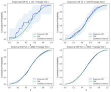
Empirical CDF, CDF and Confidence Interval plots for various sample sizes of Triangle Distribution

Statistical implementation [edit]

A non-exhaustive list of software implementations of Empirical Distribution function includes:

• In R software, we compute an empirical cumulative distribution function, with several methods for plotting, printing and computing with such an "ecdf" object.
• In MATLAB we can use Empirical cumulative distribution function (cdf) plot
• jmp from SAS, the CDF plot creates a plot of the empirical cumulative distribution function.
• Minitab, create an Empirical CDF
• Mathwave, we can fit probability distribution to our data
• Dataplot, we can plot Empirical CDF plot
• Scipy, using scipy.stats we can plot the distribution
• Statsmodels, we can use statsmodels.distributions.empirical_distribution.ECDF
• Matplotlib, we can use histograms to plot a cumulative distribution
• Seaborn, using the seaborn.ecdfplot function
• Plotly, using the plotly.express.ecdf function
• Excel, we can plot Empirical CDF plot

See also [edit]

• Càdlàg functions
• Count data
• Distribution fitting
• Dvoretzky–Kiefer–Wolfowitz inequality
• Empirical probability
• Empirical process
• Estimating quantiles from a sample
• Frequency (statistics)
• Kaplan–Meier estimator for censored processes
• Survival function
• Q–Q plot

References [edit]

1. ^ A modern introduction to probability and statistics : understanding why and how. Michel Dekking. London: Springer. 2005. p. 219. ISBN978-1-85233-896-1. OCLC 262680588. {{cite book}}: CS1 maint: others (link)
2. ^ ^{a b c} van der Vaart, A.W. (1998). Asymptotic statistics . Cambridge University Press. p. 265. ISBN0-521-78450-6.
3. ^ PlanetMath Archived May 9, 2013, at the Wayback Machine
4. ^ Coles, S. (2001) An Introduction to Statistical Modeling of Extreme Values. Springer, p. 36, Definition 2.4. ISBN 978-1-4471-3675-0.
5. ^ Madsen, H.O., Krenk, S., Lind, S.C. (2006) Methods of Structural Safety. Dover Publications. p. 148-149. ISBN 0486445976
6. ^ ^{a b} van der Vaart, A.W. (1998). Asymptotic statistics . Cambridge University Press. p. 266. ISBN0-521-78450-6.
7. ^ ^{a b c} van der Vaart, A.W. (1998). Asymptotic statistics . Cambridge University Press. p. 268. ISBN0-521-78450-6.

Further reading [edit]

• Shorack, G.R.; Wellner, J.A. (1986). Empirical Processes with Applications to Statistics. New York: Wiley. ISBN0-471-86725-X.

External links [edit]

• Media related to Empirical distribution functions at Wikimedia Commons

davishendes70.blogspot.com

Source: https://en.wikipedia.org/wiki/Empirical_distribution_function

Share this post